Introduction
Google Maps and Google Earth (hereafter Google Maps) are publicly available tools useful to visually explore the geography of our planet. Globally distributed high resolution satellite data are used as a background to dynamically map physical, geographical, historical, socio-economic or political thematic layers. Nowadays the average, educated person with access to the internet either interactively applies Google Maps for commercial or private activities or passively uses it through media coverage. Hence, the perception of the earth’s visual appearance is successively becoming based on this particular data source.
Google Maps have a highly advanced interface for simultaneously merging and displaying a complex set of data sources. The thematic layers of Google Maps are accurate and they often include real-time information. The background imagery, however, lacks some level of realism, identified here as a weak treatment of the underlying satellite data. Scientific and technical methods were for instance developed and applied in NASA’s Blue Marble Next Generation project (hereafter BMNG, http://bluemarble.nasa.gov) to correct for such issues, and they could serve as a guideline to improve Google Maps. The aim of the following discussion is therefore to outline a few methods that could yield better spatial consistency of the satellite data used in Google Maps. It is important for educational and scientific purposes that the public perceives a realistic view of our planet.
The discussion is accompanied by the following slides, presented by me in a video conference at Google Zurich on 28 February 2012.
Problem Description
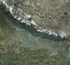
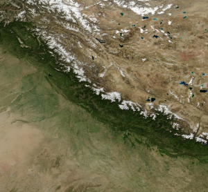
Google Maps offer amazing detail when viewed at the street, city and landscape scale. However, regional and continental views of our planet often appear rather discontinuous as a patchwork of different satellite scenes and as a mix of true and false color composites. Problematic regions also include those with a distinct seasonality such as temperate and boreal climates, regions with heavy cloudiness such as the tropics, and regions with high aerosol loads such as areas with biomass burning or with urban pollution.
Most discontinuities are a result of stitching temporally discontinuous satellite datasets with differing atmospheric disturbances, directional effects of the sun-earth-satellite viewing geometry, spectral differences between satellite sensors and last but not least the seasonal differences of the earth surface’s vegetation and snow cover. Most of these effects can be overcome if suitable satellite remote sensing algorithms are applied. We have demonstrated it for the BMNG at 500 m spatial resolution (Stöckli et al. 2005).
Possible Solutions
In order to carry out a similar set of corrections for Google Maps, fundamental processing of satellite data using well established algorithms could firstly be applied to the satellite scenes used for Google Maps. Secondly, novel methods would have to be developed in order to optimizespatio-temporal compositing of those satellite scenes.
1) Scene Processing
The aim of scene processing is to retrieve the surface reflectance (visible and near-infrared spectral bands) or brightness temperature (infrared spectral bands) for cloud free pixels in each satellite scene. This is mandatory for the further retrieval of physical properties from a satellite dataset. It can be applied to most satellite sensors, including those used for Google Maps (e.g. Landsat, SPOT and probably even to GeoEye, Worldview and QuickBird). Scene processing can be computationally expensive but mature algorithms are publicly available from the science community (for instance the LEDAPS code; Masek et al. 2006). Scene processing requires the existence of level 1 or 1b satellite data including extensive metadata (like sensor calibration, geographic registration, satellite radiances etc.). Processed satellite images or image composites cannot be used for physical retrievals and corrections.
The following steps (among others) are carried out during scene processing:
- registration & navigation
- removal of geometric and radiometric artifacts
- orthorectification
- radiance (inter-) calibration degraded sensors (de Vries et al. 2007)
- cloud masking (Khlopenkov and Trishchenko 2007)
- correction of atmospheric effects (Vermote et al. 2002)
- spectral conversion to pre-defined bands
Scene processing can yield cloud-free surface reflectances that also include per-pixel estimates of the retrieval error. This error can be defined heuristically from quality flags of each processing step. It can also be estimated by using bayesian algorithms, such as for instance a cloud mask based on an optimal estimation technique. Retrieval errors are an important input for scene compositing, where the clear sky surface reflectances are used for the estimation of model parameters.
2) Scene Compositing
The aim of scene compositing is to achieve spatial consistency by merging the corrected and masked scenes from above processing in time and space. Simple spatial stitching methods are often used, but they cannot provide spatial consistency. Often, neighboring scenes are from a different season or year and they do neither match solar illumination geometry nor the highly variable state of surface. A composite will then have visible boundaries where stitching took place. A better result can be achieved by temporal compositing from a stack of seasonally distributed scenes of the same area of interest. The composite for a given pixel, date, solar and view geometry is then calculated by use of a time series analysis approach. This requires the availability of satellite data with a high enough temporal revisit frequency (every month or less), or with long enough temporal coverage (many years of observation).
The following steps (among others) are required for scene compositing:
- calculate surface BRDF effects
- calculate seasonal dynamics of vegetation
- remove gaps with temporal interpolation
All three steps are best calculated together in one single algorithm since they involve the inversion of semi-empirical models where 3-10 parameters have to be fitted to each pixel. The parameter space often is characterized by a high order of equifinality, thus the minimization of the involved cost function is not trivial. The simplest approach uses 2nd and 3rd order Fourier series and yields a mixed retrieval of BRDF and seasonality based on 2-3 parameters per pixel. If a BRDF model and a phenology model are both available, an optimal estimation or ensemble-based bayesian data assimilation could be applied to retrieve 6-8 parameters per pixel (Stöckli et al. 2011). In case of a poor temporal coverage, multi-sensor parameter estimation may be applied. This for instance means that a landcover-dependent set of BRDF parameters is firstly estimated at MODIS pixel scale. MODIS-based parameters are then down-scaled and applied to Landsat or SPOT resolution (Li et al. 2010).
Conclusions and Outlook
The key ideas outlined above are that scene compositing employs the temporal domain to guarantee consistency of the resulting composite in the spatial domain. The underlying data source has to be properly processed beforehand, and it needs to have a high enough temporal coverage. Such a framework has been successfully applied in the generation of the BMNG dataset. With little or no spatial dependencies involved, the required computations, specifically the model inversions for parameter estimation, can be parallelized very efficiently.
What has worked for the BMNG using MODIS data does not necessarily have to be applicable to other satellite data. NASA’s MODIS sensor offered well-calibrated data at a high temporal revisit frequency and the MODIS science team guaranteed that scene processing was carried out with state-of-the-art algorithms. The scene compositing employed for the BMNG project was therefore based on data that fulfilled very high technical and scientific standards.
In order to find out how Landsat and SPOT based global satellite composites could be generated, the following questions would need to be answered:
- What kind of processing and compositing is applicable to the Landsat and SPOT satellite data (inventory of data sources)?
- What kind of processing and compositing can be readily applied and yield good improvements (low hanging fruit)?
- Which processing and compositing step would yield high improvements at a high investment (exceptionally sweet but high hanging fruit?)
- Which scene processing has already been applied to Landsat and SPOT data (inventory of methods)?
- Which scene compositing has already been applied to Landsat and SPOT data (inventory of methods)?
- Which scientific and technical methods are available and have been successful (literature review)?
- What are the most wanted user requirements (prioritize tasks)?
- Which are the geographic areas that need most attention (prioritize region)?
- Has anything similar been done at the MODIS, SPOT, Landsat science team (harvest knowledge, avoid duplication)?
Based on such an “inventory” a strategy could then be generated for how to improve, what to improve and where to improve at what cost. Even a partial execution of scene processing and compositing could result in a substantial improvements of the Landsat and SPOT based satellite layer used in Google Maps.
References
R. Stöckli, E. Vermote, N. Saleous, R. Simmon, and D. Herring. True color earth data set includes seasonal dynamics. EOS, 87(5):49, 55, 2006.
R. Stöckli, T. Rutishauser, I. Baker, M. Liniger, and A. S. Denning. A global reanalysis of vegetation phenology. J. Geophys. Res. – Biogeosciences, 116(G03020), 2011. doi: 10.1029/2010JG001545.
F. Li, D. L. B. Jupp, S. Reddy, L. Lymburner, N. Mueller, P. Tan, and A. Islam. An evaluation of the use of atmospheric and brdf correction to standardize landsat data. Ieee Journal of Selected Topics In Applied Earth Observations and Remote Sensing, 3(3):257–270, Sept. 2010. doi: 10.1109/JSTARS.2010.2042281.
C. de Vries, T. Danaher, R. Denham, P. Scarth, and S. Phinn. An operational radiometric calibration procedure for the landsat sensors based on pseudo-invariant target sites. Remote Sensing of Environment, 107(3):414–429, Apr. 2007. doi: 10.1016/j.rse.2006.09.019.
E. F. Vermote, N. Z. E. Saleous, and C. O. Justice. Atmospheric correction of MODIS data in the visible to middle infrared: first results. Remote Sens. Environ., 83:97–111, 2002.
J. Masek, E. Vermote, N. Saleous, R. Wolfe, F. Hall, K. Huemmrich, F. Gao, J. Kutler, and T. Lim. A landsat surface reflectance dataset for north america, 1990-2000. Ieee Geoscience and Remote Sensing Letters, 3 (1):68–72, Jan. 2006. doi: 10.1109/LGRS.2005.857030.
K. V. Khlopenkov and A. P. Trishchenko. Sparc: New cloud, snow, and cloud shadow detection scheme for historical 1-km avhhr data over canada. J Atmos Oceanic Tech, 24(3):322–343, Jan 2007. doi: 10.1175/JTECH1987.1.


