… is not my business. But anyway …


Apr 20 2018
The Buttkicker Simulation Kit has arrived. After being sold out for years it is finally available again. It’s a fine piece of hardware. Connecting is easy. I’ve screwed the Transducer under the original B737 seat and it makes a difference during flight.
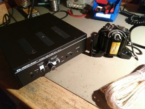

What is needed now would be to add low frequency vibrations to individual flight systems such as landing gear, flaps or for environmental influences such as turbulence or ground contact. The low frequency vibrations are only partly realistic through the original X-Plane sounds.
Apr 20 2018
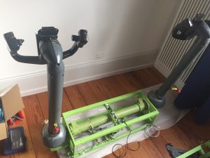
It took some time to rebuild the cockpit so that it would fit the simujabs control column and rudder pedal mechanics. The whole construction had to be raised by around 22 cm which enabled placing the column and rudder mechanics under the “double floor”. The result is fantastic. See yourself …


Above images show the rudder mechanics of simujabs. They are linked and controlled by regular springs. The toe brakes are controlled by gas springs. One of the difficulties was to add both sets of toe brakes to X-Plane since X-Plane only has functionality for one left and one right toe brake (my guess is that this corresponds to how it works in a plane … toe brakes are linked as well?!). So the solution was to send their inputs to usbiocards() and send the max() of both left and both right brakes to X-Plane by TCP/IP and the xpserver() plugin.


Here it goes and the stuff seems to fit in my small unheated attic just below the roof.


The double floor construction raises the platform by around 22 cm and fits the rudder and yoke column mechanics nicely below the “hood”.


Connecting all the wires including the original Boeing 737 column buttons etc took some time and guess what … those original yokes are double wired everywhere (for safety), so I could add some more functionality like the 4-way hat switch replacing the 3 digit dial on the Yoke. This hat switch comes in handy for switching views without having to access the computer keyboard. The hat switch is an APEM HS1A14SA 4-way switch. Next time I’d order one with the included pushbutton.


The roll mechanism centers well enough although there is some slackness between the two yokes during rotation due to all the mechanical 90 degree connections between them.


The interesting fact is that I had to re-learn how to fly with those original columns and rudder pedals. I havea used a joystick and CH Rudder Pedals for years where small movements with each hand or leg or toe make the difference. With the originals mounted there is both force and physical movement needed to control the plane. Lot’s of fun.
Dec 21 2017
To enhance a home cockpit with realistic controls instead of just using a simple joystick and gaming rudder pedals is possibly the dream of every cockpit builder. So here it goes …
Boeing Airliners still have *real* linked Yoke Columns and Rudder Pedals. And there is quite some mechanical engineering involvend when you want to re-build them at home. So, I was first of all lucky to get a pair of real Boeing 737-300 control columns including the linking crossover bar from my colleague Jim Doyle of Desert Air Spares. The good thing is that those heavy and proven parts have not really changed much throughout the Boeing 737 history. So the NG’s still use almost the same model as did the -200’s 40 years ago. This is not a sign of laziness on the side of Boeing but a sign of good quality and of a working concept. However, the control crossover bar was not complete, there were one 10 cm part missing and both bearings were missing as well. Now it is not that simple to get those parts on the free market. Most cockpits of used airliners get sold in one piece nowadays to cockpit builders like me. The FAA-certified spare parts on the other hand are available but they come with a quite fancy price tag. And who needs FAA-certified parts for a plane that will never fly, anyway …
Jim helped me to get in contact with several companies and finally the parts were available and delivered from Universal Asset Management (UAM INC).


Having the original parts at hand means first of all a lot of joy but at the same time some real trouble: how to mount them, they are really heavy. This is where the real work starts. And I am very glad to have met Pedro Bibiloni which owns SimuJabs, located in Mallorca Spain. Neither being a trained mechanic nor having any of the required tools for serious metal work this contact saved my life (I cannot say it differently). I have looked around for other companies which offer dual linked Boeing 737 control columns but none of them seemed either as professional as Simujabs nor do they seem have the required frames to fit the heavy original parts.
Pedro offered me to adapt one of his motorized yoke column frame to fit the original parts. The process involved Pedro asking me for the exact measures of just about every corner of these original parts. He actually suggested that I could send the columns to Mallorca and he would do the job. But at the end we agreed that we do it all by trusting each other and by very good imagination of each other’s descriptions.
This October two really large packages arrived. Mounting the yoke columns and the crossover bar was a great experience with the high precision work done by Pedro. The only thing which we realized was that the absolute distance between the columns is not 1020 mm as communicated by MarkusPilot but 1017 mm. You might now think that this is a real detail, but 3 mm’s are a big deal when it comes to link the roll mechanism between the two columns.

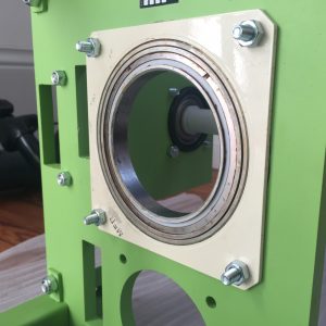
The roll mechanism in the SimuJabs construction is a highly advanced ball joint (left picture below) with the joint exactly at the center of the pitch axis rotation (right picture below). The roll force is then transferred under the crossover bar by chains, roll force regulated by regular springs. The pitch rotation is regulated by heavy duty gas springs sitting at the top of the frame (can be seen in the right picture above).

Pedro from SimuJabs also delivered a pair of standard linked rudder pedals with all the bells and whistles. They work great! The only thing that I have to find out is how to assign two sets of toe brakes (Captain and First Officer separately) to the X-Plane control inputs. In X-Plane there is only one set of toe brakes allowed.
More on the exclusive and professional rudder pedals of SimuJabs in a next post.
Conclusion
If you ever need a professional set of linked Yoke Columns or Rudder Pedals, please count on SimuJabs.
Dec 18 2017
Back in 2004 I started to think about how I could build a real airliner cockpit entirely based on Linux. I At the end of 2017 (and with a grown family) this idea has evolved into a fun project. The way to that goal is still a long and a very creative one. But today I can share first of all a few specifications of how I proceeded with it and you will find a few images documenting the current status of my Boeing 737-800 (NG) home cockpit.
The first thing to think about when running linux is which flight simulator to pick. The number of candidates is barely countable … For entirely open source fanatics Flight Gear would be the way to go. However, X-Plane was my choice because of its highly sophisticated aerodynamics and visual simulation quality. And X-Plane is extendable on just about every side.
The second thing to think about is how to connect hardware to your Linux box and to the flight simulator itself, and then, which hardware to pick (or vice versa). Hardware there is much. But all available software interfaces are written for Windows-based flight simulators and most of them again for the Microsoft Flight Simulator itself. I have chosen the famous OpenCockpits set of I/O cards for my project and extended it with Leo Bodnar‘s even ore famous joystick and I/O cards.
The way to go was to invent my own interface to OpenCockpits and Leo Bodnar’s I/O cards. I call it xpiocards and it is managed as open source together with my colleague Hans who joins my linux home cockpit fate with his Airbus A320 cockpit. The difficult part was to reverse engineer the not-so-open Open Cockpits hardware communication (the blueprints are open, but the communication protocol is not). This yielded a highly stable USB communication to the client application usbiocards and to a even more stable TCP/IP communication to the xpserver server plugin in X-Plane. Since all the code is custom made I have full control over all issues and can correct bugs on the fly. This is not the case if you build a home cockpit with proprietary flight software. Isn’t it fun to have control over something so complex which is only enjoyable if your flight experience is free of glitches … especially at the last 100 feet prior to a difficult landing?
The great part of the current server client I/O application is that there is no need to manually edit plugin-side dataref list which is exchanged with the clients (in FSUIPC language: defining a list of offsets). The client (in fact any number of clients) simply subscribe to their specific datarefs which are then sent to them in regular intervals. In fact they are only sent if they are updated on the flight simulator side or updated on the client side. Isn’t this a marvellous idea? No need to exchange unnessesary data …


It all started with a few X-Plane datarefs being exchanged between X-Plane and a simple NAV radio panel based on OpenCockpits hardware. I have bought the I/O cards and panels and built the electronics myself. The weak part of OpenCockpits is the uneven backlighting capability and the “not so open” communication protocol of their I/O Cards.
A big progress has happened once my colleague Torsten from CockpitForYou has delivered the motorized B737 Throttle Quadrant. The package was huge and I had to get it from the cargo company office … since I do not own a car the picture above tells you how it can be done with our kids trailer: it is also a cargo bike!


The next great step forward was to complete the full B737 pedestal. For this Lausitz Aviation delivered a highly professional pedestal case in which I could mount the Open Cockpits panels and the underlying electronics.


The current final task was to mount a 55″ TV and also integrate and further develop the outdated OpenGC code into a fully functional Boeing 737 Primary Flight Display (PFD), Navigation Display (NAV) and Engine Indication and Crew Alterting System (EICAS) set of displays on a second monitor.
And yes: the best of all. My colleague Benedikt Stratmann from EADT is building the same beautiful plane with its full functionality by software as I am by hardware. So here you go: a big applause for EADT and their famous x737. You see the airplane above with the Air Greenland livery stationed at the Marina di Campo airport on the Elba island.
So here you get a list on the current hardware / software setup:
And watch out for more. The flight controls are in progress …
Apr 26 2016
The Swiss Federal Office of Energy SFOE, the Federal Office of Meteorology and Climatology MeteoSwiss, and the Federal Office of Topography swisstopo have created together with Meteotest a stunningly interactive and publicly accessible solar potential estimator for whole Switzerland.

Solar Potential Map of Switzerland
Compared to traditional so-called GIS-type “solar cadasters” this one is really usable. By usable I mean:

One click to the solar yield calculation of your roof!
I’m of course a bit biased since I created and provided the satellite-based solar irradiance data to the project as part of my engagement within MeteoSwiss. But try it out yourself!
Jan 11 2015
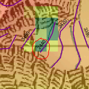
By analysis of our MeteoSwiss high quality satellite-based solar irradiance maps created by the Heliomont algorithm I’ve found that the sunniest place in Switzerland is close to the Monte Rosa hut of the Swiss Alpine Club SAC. During the calculation of the Solar Atlas of Switzerland (to be published as “The Solar Cadaster of Switzerland” on the Geoportal of the Swiss Government) I have also detected the absolutely DARKEST spot in Switzerland. Here it is:
The point lies at 636125 / 93050 (CH1903 / LV03 coordinate system) at the border between Switzerland and Italy. It has as sky view factor of 0.003. This is about the same sky view as found in a bottomless pit. There is no solar irradiance getting down there. The yearly mean solar irradiance is around 0.5 W m-2 (Watts per square meter; the average over most of Switzerland is well over 150 W m-2). The reason for this low predicted solar irradiance can be found in the Swiss elevation model DHM 25 at the spatial resolution of 25 m. These are the topographic elevations (m) of the darkest point including its 8 neighboring points:
2996 2622 3414
2763 2440 3457
3070 3131 3484
The center point lies between 200 – 1000 m lower than the surrounding grid points. Is this bottomless pit in beautiful landscape reality or a digital artifact?
Update
The customer service of SwissTopo has kindly provided a credible answer: The darkest spot is indeed an artifact of the DHM25 dataset due to a contour line which was digitized 1000 m below its actual elevation:
May 24 2012
 During the last few decades flowering and leafing of temperate and boreal vegetation has advanced by several days in response to warming. The climate sensitivity, as inferred from long-term observations, is estimated to be 2.5-5.0 days per degree C warming. Wolkovich et al. now show in their letter to Nature, that this response cannot be replicated in field experiments where vegetation is artificially warmed: in these experiments the warming effect on vegetation phenology is 4.0-8.5 times lower than in long-term observations:
E. M. Wolkovich, B. Cook, J. Allen, T. Crimmins, J. Betancourt, S. Travers, S. Pau, J. Regetz, T. Davies, N. Kraft, T. Ault, K. Bolmgren, S. Mazer, G. McCabe, B. McGill, C. Parmesan, N. Salamin, M. Schwartz, and E. Cleland. Warming experiments underpredict plant phenological responses to climate change. Nature, 485:494–497, 2012. doi: 10.1038/nature11014.
Two author teams, This Rutishauser and I, and John Harte and Lara Kueppers, have been invited to comment the letter by Wolkovich et al. Our comment was published today in the same issue of Nature:
T. Rutishauser, R. Stöckli, J. Harte, and L. Kueppers. Climate change: Flowering in the greenhouse. Nature, 485:448–449, 2012. doi: 10.1038/485448a. [PDF]
We conclude and suggest:
– Temperature effects are not independent from effects of other environmental changes
– Phenology is much more than a linear correlate to annual mean air temperatures
– Wolkovich’s call for ecosystem model re-evaluation has to be taken seriously
Finally, a very interesting question arises from the work by Wolkovich et al.:
“Are temperature sensitivities derived from past phenological observations valid for application in a future, warmer climate?”
We haven’t found the answer in the scientific literature (yet!).
Sincerely,
Reto and This
May 04 2012
![]()
Digital Object Identifiers (DOI’s) are often used to uniquely identify and reference digital content of written documents such as scientific publications or books. This is helpful to track a content over a long time period, where the actual location of the content may change, but any reference to it will have to stay the same.
DOI’s are not just suitable for electronic documents but in fact for any digital content. We have now created a DOI for our long term satellite-based Surface Radiation MVIRI Dataset from the Satellite Application Facility on Climate Monitoring by Rebekka Posselt, Richard Müller, Reto Stöckli and Jörg Trentmann (2011):